How to add vertical line to line chart in Excel

How to add vertical line to Excel chart: scatter plot, bar chart and line graph

To insert a vertical line in a line graph, you can use either of the previously described techniques. For me, the second method is a bit faster, so I will be using it for this example. Additionally, we will make our graph interactive with a scroll bar:

Insert vertical line in Excel graph

To add a vertical line to an Excel line chart, carry out these steps:

1. Select your source data and make a line graph (Inset tab > Chats group > Line).
2. Set up the data for the vertical line in this way:
   • In one cell (E1), type the text label for the data point at which you want to draw a line exactly as it appears in your source data.
   • In two other cells (D3 and D4), extract the X value for the target data point by using this formula:
   =IFERROR(MATCH($E$1,$A$2:$A$7,0), 0)The MATCH function returns the relative position of the lookup value in the array, and the IFERROR function replaces a potential error with zero when the lookup value is not found.
   • In two adjacent cells (E3 and E4), enter the Y values of 0 and 1.
   With the vertical line data in place, please follow steps 3 – 13 from the bar chart example to plot a vertical line in your chart. Below, I will briefly walk you through the key points.
3. Right-click anywhere in the chart, and then click Select Data… .
4. In the Select Data Source dialogue box, click the Add button.
5. In the Edit Series window, type any name you want in the Series name box (e.g. Vertical Line), and select the cells with X values for the Series values box (D3:D4 in our case).
   
6. Right click anywhere in the chart and choose Change Chart Type from the pop-up menu.
7. In the Change Chart Type window, make the following changes:
   • On the All Charts tab, select Combo.
   • For the main data series, choose the Line chart type.
   • For the Vertical Line data series, pick Scatter with Straight Lines and select the Secondary Axis checkbox next to it.
   • Click OK.
8. Right-click the chart and choose Select Data…
9. In the Select Data Source dialog box, select the Vertical Line series and click Edit.
   
10. In the Edit Series dialog box, select the X and Y values for the corresponding boxes, and click OK twice to exit the dialogs.
    
11. Right-click the secondary y-axis on the right, and then click Format Axis.
12. On the Format Axis pane, under Axis Options, type 1 in the Maximum bound box to ensure that your vertical line extends to the top of the chart.
13. Hide the right y-axis by setting Label Position to None.

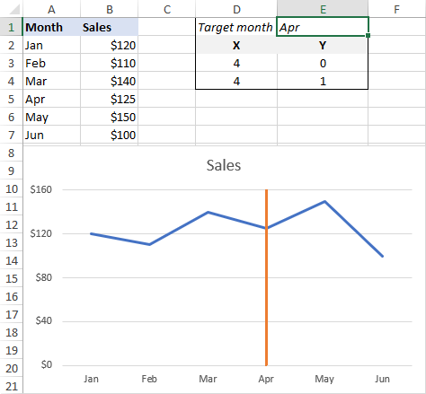
Your chart with a vertical line is done, and now it’s time to try it out. Type another text label in E2, and see the vertical line move accordingly.

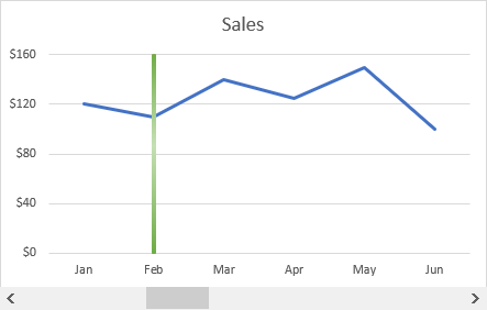
Don’t want to bother typing? Fancy up your graph by adding a scroll bar!

Make a vertical line interactive with a scroll bar

To interact with the chart directly, let’s insert a scroll bar and connect our vertical line to it. For this, you will need the Developer Tab. If you don’t have it on your Excel ribbon yet, it is very easy to enable: right-click the ribbon, click Customize Ribbon, select Developer under Main Tabs, and click OK. That’s it!

And now, perform these simple steps to insert a scroll bar:

1. On the Developer tab, in the Controls group, click the Insert button, and then click Scroll Bar under Form Controls:
   
2. On top or at the bottom of your graph (depending on where you want the scroll bar to appear), draw a rectangle of the desired width using the mouse. Or simply click anywhere on your sheet, and then move and resize the scroll bar as you see fit.
3. Right click the scroll bar and click Format Control….
   
4. Link your scroll bar to some empty cell (D5), set the Maximum Value to the data points total and click OK. We have data for 6 months, so we set the Maximum Value to 6.
   
5. The linked cell now shows the value of the scroll bar, and we need to pass that value to our X cells in order to bind the vertical line to the scroll bar. So, delete the IFERROR/MATCH formula from cells D3:D4 and enter this simple one instead: =$D$5

The Target month cells (D1 and E1) are not needed any longer, and you are free to delete them. Or, you can return the target month by using the below formula (which goes to cell E1):

=IFERROR(INDEX($A$2:$A$7, $D$5, 1), "")

That’s it! Our interactive line chart is completed. That has taken quite a bit of time, but it’s worth it. Do you agree?

That’s how you create a vertical line in Excel chart. For hands-on experience, please feel free to download our sample workbook below. I thank you for reading and hope to see you on our blog next week!